Fourier Transform
Note
We assume that by now you have already read the previous tutorials. If not, please check previous tutorials at http://opencv-java-tutorials.readthedocs.org/en/latest/index.html. You can also find the source code and resources at https://github.com/opencv-java/
우리는 지금까지 이미 이전 튜토리얼을 읽었다 고 가정합니다. 그렇지 않은 경우 http://opencv-java-tutorials.readthedocs.org/en/latest/index.html에서 이전 자습서를 확인하십시오. https://github.com/opencv-java/에서 소스 코드와 리소스를 찾을 수도 있습니다.
Goal
In this tutorial we are going to create a JavaFX application where we can load a picture from our file system and apply to it the DFT and the inverse DFT.
이 튜토리얼에서는 파일 시스템에서 그림을로드하고 DFT와 역 DFT를 적용 할 수있는 JavaFX 애플리케이션을 작성하려고합니다.
In this tutorial we are going to create a JavaFX application where we can load a picture from our file system and apply to it the DFT and the inverse DFT.
이 튜토리얼에서는 파일 시스템에서 그림을로드하고 DFT와 역 DFT를 적용 할 수있는 JavaFX 애플리케이션을 작성하려고합니다.
What is the Fourier Transform?
The Fourier Transform will decompose an image into its sinus and cosines components. In other words, it will transform an image from its spatial domain to its frequency domain. The result of the transformation is complex numbers. Displaying this is possible either via a real image and a complex image or via a magnitude and a phase image. However, throughout the image processing algorithms only the magnitude image is interesting as this contains all the information we need about the images geometric structure. For this tutorial we are going to use basic gray scale image, whose values usually are between zero and 255. Therefore the Fourier Transform too needs to be of a discrete type resulting in a Discrete Fourier Transform (DFT). The DFT is the sampled Fourier Transform and therefore does not contain all frequencies forming an image, but only a set of samples which is large enough to fully describe the spatial domain image. The number of frequencies corresponds to the number of pixels in the spatial domain image, i.e. the image in the spatial and Fourier domain are of the same size.
푸리에 변환은 이미지를 부채꼴 및 코사인 구성 요소로 분해합니다. 즉, 이미지를 공간 영역에서 주파수 영역으로 변환합니다. 변환의 결과는 복소수입니다. 이것을 표시하는 방법은 실제 이미지와 복잡한 이미지 또는 크기 및 위상 이미지를 통해 가능합니다. 그러나 이미지 처리 알고리즘 전체에 걸쳐 크기 이미지 만 흥미 롭습니다. 여기에는 이미지 기하 구조에 대해 필요한 모든 정보가 포함되어 있기 때문에 흥미 롭습니다. 이 튜토리얼에서 우리는 값이 보통 0과 255 사이의 기본 회색조 이미지를 사용할 것입니다. 따라서 푸리에 변환 역시 이산 푸리에 변환 (Discrete Fourier Transform, DFT)의 결과를 가져야합니다. DFT는 샘플링 된 푸리에 변환이므로 이미지를 형성하는 모든 주파수를 포함하지는 않지만 공간 도메인 이미지를 완전히 설명하기에 충분히 큰 샘플 세트 만 포함합니다. 주파수의 수는 공간 도메인 이미지의 픽셀의 수에 상응한다. 즉, 공간 및 푸리에 도메인의 이미지는 동일한 크기이다.
What we will do in this tutorial
- In this guide, we will:
- Load an image from a file chooser.
- Apply the DFT to the loaded image and show it.
- Apply the iDFT to the transformed image and show it.
이 가이드에서 우리는 :파일 선택기에서 이미지를로드하십시오.로드 된 이미지에 DFT를 적용하고 표시합니다.변환 된 이미지에 iDFT를 적용하고 보여줍니다.
- In this guide, we will:
- Load an image from a file chooser.
- Apply the DFT to the loaded image and show it.
- Apply the iDFT to the transformed image and show it.
이 가이드에서 우리는 :파일 선택기에서 이미지를로드하십시오.로드 된 이미지에 DFT를 적용하고 표시합니다.변환 된 이미지에 iDFT를 적용하고 보여줍니다.
Getting Started
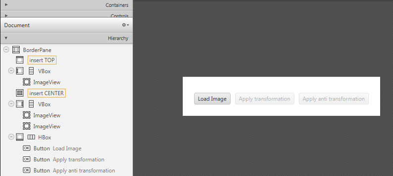
Let’s create a new JavaFX project. In Scene Builder set the windows element so that we have a Border Pane with:
새로운 JavaFX 프로젝트를 만들어 보겠습니다. Scene Builder에서 windows 요소를 설정하여 다음과 같은 테두리 창을 갖도록하십시오.
- on the LEFT an ImageView to show the loaded picture:
왼쪽에로드 된 그림을 보여주는 ImageView :
<ImageView fx:id="originalImage" />
- on the RIGHT two ImageViews one over the other to display the DFT and the iDFT;
DFT와 iDFT를 표시하려면 오른쪽에 두 개의 ImageViews 하나를 다른 하나에;
<ImageView fx:id="transformedImage" />
<ImageView fx:id="antitransformedImage" />
- on the BOTTOM three buttons, the first one to load the picture, the second one to apply the DFT and show it, and the last one to apply the anti-transform and show it.
BOTTOM 버튼 세 개, 그림을로드하는 첫 번째 버튼, DFT를 적용하고 보여줄 두 번째 버튼, 반 변환을 적용하고 보여주기위한 마지막 버튼.
<Button alignment="center" text="Load Image" onAction="#loadImage"/>
<Button fx:id="transformButton" alignment="center" text="Apply transformation" onAction="#transformImage" disable="true" />
<Button fx:id="antitransformButton" alignment="center" text="Apply anti transformation" onAction="#antitransformImage" disable="true" />
The gui will look something like this one:
GUI는 다음과 같이 보입니다.
Let’s create a new JavaFX project. In Scene Builder set the windows element so that we have a Border Pane with:
새로운 JavaFX 프로젝트를 만들어 보겠습니다. Scene Builder에서 windows 요소를 설정하여 다음과 같은 테두리 창을 갖도록하십시오.
- on the LEFT an ImageView to show the loaded picture:
<ImageView fx:id="originalImage" />
- on the RIGHT two ImageViews one over the other to display the DFT and the iDFT;
<ImageView fx:id="transformedImage" />
<ImageView fx:id="antitransformedImage" />
- on the BOTTOM three buttons, the first one to load the picture, the second one to apply the DFT and show it, and the last one to apply the anti-transform and show it.
<Button alignment="center" text="Load Image" onAction="#loadImage"/>
<Button fx:id="transformButton" alignment="center" text="Apply transformation" onAction="#transformImage" disable="true" />
<Button fx:id="antitransformButton" alignment="center" text="Apply anti transformation" onAction="#antitransformImage" disable="true" />
The gui will look something like this one:
GUI는 다음과 같이 보입니다.
Load the file
First of all you need to add to your project a folder resources with two files in it. One of them is a sine function and the other one is a circular aperture. In the Controller file, in order to load the image to our program, we are going to use a filechooser:
먼저 프로젝트에 두 개의 파일이있는 폴더 리소스를 추가해야합니다. 그 중 하나는 사인 함수이고 다른 하나는 원형 구경입니다. 컨트롤러 파일에서 이미지를 프로그램에로드하려면 filechooser를 사용합니다.
private FileChooser fileChooser;
When we click the load button we have to set the initial directory of the FC and open the dialog. The FC will return the selected file:
로드 버튼을 클릭하면 FC의 초기 디렉토리를 설정하고 대화 상자를 열어야합니다. FC가 선택한 파일을 반환합니다.
File file = new File("./resources/");
this.fileChooser.setInitialDirectory(file);
file = this.fileChooser.showOpenDialog(this.main.getStage());
Once we’ve loaded the file we have to make sure that it’s going to be in grayscale and display the image into the image view:
파일을로드하고 나면 그 파일이 회색 음영으로 표시되고 이미지를 이미지보기에 표시해야합니다.
this.image = Imgcodecs.imread(file.getAbsolutePath(), Imgcodecs.CV_LOAD_IMAGE_GRAYSCALE);
this.originalImage.setImage(this.mat2Image(this.image));
Applying the DFT
First of all expand the image to an optimal size. The performance of a DFT is dependent of the image size. It tends to be the fastest for image sizes that are multiple of the numbers two, three and five. Therefore, to achieve maximal performance it is generally a good idea to pad border values to the image to get a size with such traits. The getOptimalDFTSize() returns this optimal size and we can use the copyMakeBorder() function to expand the borders of an image:
우선 이미지를 최적의 크기로 확장합니다. DFT의 성능은 이미지 크기에 따라 다릅니다. 숫자 2, 3 및 5의 배수 인 이미지 크기에서 가장 빠른 경향이 있습니다. 따라서 최대 성능을 얻으려면 일반적으로 이미지에 테두리 값을 덧붙여 이러한 특성을 가진 크기를 얻는 것이 좋습니다. getOptimalDFTSize ()는이 최적의 크기를 반환하고 copyMakeBorder () 함수를 사용하여 이미지의 테두리를 확장 할 수 있습니다.
int addPixelRows = Core.getOptimalDFTSize(image.rows());
int addPixelCols = Core.getOptimalDFTSize(image.cols());
Core.copyMakeBorder(image, padded, 0, addPixelRows - image.rows(), 0, addPixelCols - image.cols(),Imgproc.BORDER_CONSTANT, Scalar.all(0));
The appended pixels are initialized with zeros.
추가 된 픽셀은 0으로 초기화됩니다.
The result of the DFT is complex so we have to make place for both the complex and the real values. We store these usually at least in a float format. Therefore we’ll convert our input image to this type and expand it with another channel to hold the complex values:
DFT의 결과는 복잡하기 때문에 복소수 값과 실수 값을 모두 계산해야합니다. 우리는 보통 float 형식으로 저장합니다. 따라서 입력 이미지를이 유형으로 변환하고 복잡한 값을 보유 할 다른 채널로 확장합니다.
padded.convertTo(padded, CvType.CV_32F);
this.planes.add(padded);
this.planes.add(Mat.zeros(padded.size(), CvType.CV_32F));
Core.merge(this.planes, this.complexImage);
Now we can apply the DFT and then get the real and the imaginary part from the complex image:
이제 DFT를 적용한 다음 복잡한 이미지에서 실수와 허수를 구할 수 있습니다.
Core.dft(this.complexImage, this.complexImage);
Core.split(complexImage, newPlanes);
Core.magnitude(newPlanes.get(0), newPlanes.get(1), mag);
Unfortunately the dynamic range of the Fourier coefficients is too large to be displayed on the screen. To use the gray scale values for visualization we can transform our linear scale to a logarithmic one:
불행히도 푸리에 계수의 동적 범위가 너무 커서 화면에 표시 할 수 없습니다. 시각화를 위해 그레이 스케일 값을 사용하기 위해 우리는 선형 스케일을 대수 스케일로 변환 할 수 있습니다 :
Core.add(Mat.ones(mag.size(), CVType.CV_32F), mag);
Core.log(mag, mag);
Remember, that at the first step, we expanded the image? Well, it’s time to throw away the newly introduced values. For visualization purposes we may also rearrange the quadrants of the result, so that the origin (zero, zero) corresponds with the image center:
첫 번째 단계에서 이미지를 확장했는지 기억하십시오. 새롭게 도입 된 가치를 버릴 시간입니다. 시각화를 위해 결과의 사분면을 재정렬하여 원점 (영, 영)이 이미지 중심에 일치하도록 할 수 있습니다.
image = image.submat(new Rect(0, 0, image.cols() & -2, image.rows() & -2));
int cx = image.cols() / 2;
int cy = image.rows() / 2;

Mat q0 = new Mat(image, new Rect(0, 0, cx, cy));
Mat q1 = new Mat(image, new Rect(cx, 0, cx, cy));
Mat q2 = new Mat(image, new Rect(0, cy, cx, cy));
Mat q3 = new Mat(image, new Rect(cx, cy, cx, cy));

Mat tmp = new Mat();
q0.copyTo(tmp);
q3.copyTo(q0);
tmp.copyTo(q3);

q1.copyTo(tmp);
q2.copyTo(q1);
tmp.copyTo(q2);
Now we have to normalize our values by using the normalize() function in order to transform the matrix with float values into a viewable image form:
이제 float 값을 가진 행렬을 볼 수있는 이미지 형식으로 변환하기 위해 normalize () 함수를 사용하여 값을 정규화해야합니다.
Core.normalize(mag, mag, 0, 255, Core.NORM_MINMAX);
The last step is to show the magnitude image in the ImageView:
마지막 단계는 ImageView에 크기 이미지를 표시하는 것입니다.
this.transformedImage.setImage(this.mat2Image(magnitude));
First of all expand the image to an optimal size. The performance of a DFT is dependent of the image size. It tends to be the fastest for image sizes that are multiple of the numbers two, three and five. Therefore, to achieve maximal performance it is generally a good idea to pad border values to the image to get a size with such traits. The getOptimalDFTSize() returns this optimal size and we can use the copyMakeBorder() function to expand the borders of an image:
우선 이미지를 최적의 크기로 확장합니다. DFT의 성능은 이미지 크기에 따라 다릅니다. 숫자 2, 3 및 5의 배수 인 이미지 크기에서 가장 빠른 경향이 있습니다. 따라서 최대 성능을 얻으려면 일반적으로 이미지에 테두리 값을 덧붙여 이러한 특성을 가진 크기를 얻는 것이 좋습니다. getOptimalDFTSize ()는이 최적의 크기를 반환하고 copyMakeBorder () 함수를 사용하여 이미지의 테두리를 확장 할 수 있습니다.
int addPixelRows = Core.getOptimalDFTSize(image.rows());
int addPixelCols = Core.getOptimalDFTSize(image.cols());
Core.copyMakeBorder(image, padded, 0, addPixelRows - image.rows(), 0, addPixelCols - image.cols(),Imgproc.BORDER_CONSTANT, Scalar.all(0));
The appended pixels are initialized with zeros.
추가 된 픽셀은 0으로 초기화됩니다.
The result of the DFT is complex so we have to make place for both the complex and the real values. We store these usually at least in a float format. Therefore we’ll convert our input image to this type and expand it with another channel to hold the complex values:
DFT의 결과는 복잡하기 때문에 복소수 값과 실수 값을 모두 계산해야합니다. 우리는 보통 float 형식으로 저장합니다. 따라서 입력 이미지를이 유형으로 변환하고 복잡한 값을 보유 할 다른 채널로 확장합니다.
padded.convertTo(padded, CvType.CV_32F);
this.planes.add(padded);
this.planes.add(Mat.zeros(padded.size(), CvType.CV_32F));
Core.merge(this.planes, this.complexImage);
Now we can apply the DFT and then get the real and the imaginary part from the complex image:
이제 DFT를 적용한 다음 복잡한 이미지에서 실수와 허수를 구할 수 있습니다.
Core.dft(this.complexImage, this.complexImage);
Core.split(complexImage, newPlanes);
Core.magnitude(newPlanes.get(0), newPlanes.get(1), mag);
Unfortunately the dynamic range of the Fourier coefficients is too large to be displayed on the screen. To use the gray scale values for visualization we can transform our linear scale to a logarithmic one:
불행히도 푸리에 계수의 동적 범위가 너무 커서 화면에 표시 할 수 없습니다. 시각화를 위해 그레이 스케일 값을 사용하기 위해 우리는 선형 스케일을 대수 스케일로 변환 할 수 있습니다 :
Core.add(Mat.ones(mag.size(), CVType.CV_32F), mag);
Core.log(mag, mag);
Remember, that at the first step, we expanded the image? Well, it’s time to throw away the newly introduced values. For visualization purposes we may also rearrange the quadrants of the result, so that the origin (zero, zero) corresponds with the image center:
첫 번째 단계에서 이미지를 확장했는지 기억하십시오. 새롭게 도입 된 가치를 버릴 시간입니다. 시각화를 위해 결과의 사분면을 재정렬하여 원점 (영, 영)이 이미지 중심에 일치하도록 할 수 있습니다.
image = image.submat(new Rect(0, 0, image.cols() & -2, image.rows() & -2));
int cx = image.cols() / 2;
int cy = image.rows() / 2;
Mat q0 = new Mat(image, new Rect(0, 0, cx, cy));
Mat q1 = new Mat(image, new Rect(cx, 0, cx, cy));
Mat q2 = new Mat(image, new Rect(0, cy, cx, cy));
Mat q3 = new Mat(image, new Rect(cx, cy, cx, cy));
Mat tmp = new Mat();
q0.copyTo(tmp);
q3.copyTo(q0);
tmp.copyTo(q3);
q1.copyTo(tmp);
q2.copyTo(q1);
tmp.copyTo(q2);
Now we have to normalize our values by using the normalize() function in order to transform the matrix with float values into a viewable image form:
이제 float 값을 가진 행렬을 볼 수있는 이미지 형식으로 변환하기 위해 normalize () 함수를 사용하여 값을 정규화해야합니다.
Core.normalize(mag, mag, 0, 255, Core.NORM_MINMAX);
The last step is to show the magnitude image in the ImageView:
마지막 단계는 ImageView에 크기 이미지를 표시하는 것입니다.
this.transformedImage.setImage(this.mat2Image(magnitude));
Applying the inverse DFT
To apply the inverse DFT we simply use the idft() function, extract the real values from the complex image with the split() function, and normalize the result with normalize():
inverse DFT를 적용하기 위해 단순히 idft () 함수를 사용하고 split () 함수로 복잡한 이미지에서 실수 값을 추출한 다음 normalize ()로 결과를 정규화합니다.
Core.idft(this.complexImage, this.complexImage);
Mat restoredImage = new Mat();
Core.split(this.complexImage, this.planes);
Core.normalize(this.planes.get(0), restoredImage, 0, 255, Core.NORM_MINMAX);
Finally we can show the result on the proper ImageView:
마지막으로 결과를 적절한 ImageView에 표시 할 수 있습니다.
this.antitransformedImage.setImage(this.mat2Image(restoredImage));
Analyzing the results
- sinfunction.png
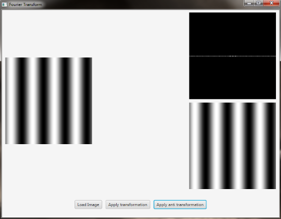
The image is a horizontal sine of 4 cycles. Notice that the DFT just has a single component, represented by 2 bright spots symmetrically placed about the center of the DFT image. The center of the image is the origin of the frequency coordinate system. The x-axis runs left to right through the center and represents the horizontal component of frequency. The y-axis runs bottom to top through the center and represents the vertical component of frequency. There is a dot at the center that represents the (0,0) frequency term or average value of the image. Images usually have a large average value (like 128) and lots of low frequency information so FT images usually have a bright blob of components near the center. High frequencies in the horizontal direction will cause bright dots away from the center in the horizontal direction.
이미지는 4 사이클의 수평 사인입니다. DFT에는 DFT 이미지의 중심을 대칭으로 배치 한 2 개의 밝은 점으로 표시되는 단일 구성 요소 만 있습니다. 이미지의 중심은 주파수 좌표계의 원점입니다. X 축은 중심을 통해 왼쪽에서 오른쪽으로 진행하며 주파수의 수평 구성 요소를 나타냅니다. y 축은 중심을 통해 아래에서 위로 실행되며 주파수의 수직 구성 요소를 나타냅니다. 중앙에는 이미지의 (0,0) 주파수 항 또는 평균값을 나타내는 점이 있습니다. 이미지는 일반적으로 큰 평균 값 (예 : 128)과 많은 저주파 정보를 가지므로 FT 이미지는 보통 중심 근처에 밝은 얼룩이 있습니다. 수평 방향으로 고주파가 발생하면 수평 방향으로 중앙에서 밝은 점들이 떨어져 나옵니다.
- circle.png
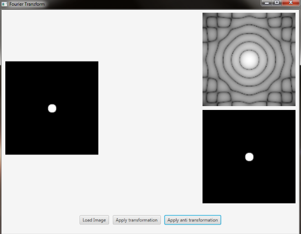
In this case we have a circular aperture, and what is the Fourier transform of a circular aperture? The diffraction disk and rings. A large aperture produces a compact transform, instead a small one produces a larger Airy pattern; thus the disk is greater if aperture is smaller; according to Fourier properties, from the center to the middle of the first dark ring the distance is (1.22 x N) / d; in this case N is the size of the image, and d is the diameter of the circle. An Airy disk is the bright center of the diffraction pattern created from a circular aperture ideal optical system; nearly half of the light is contained in a diameter of 1.02 x lamba x f_number.
이 경우 원형 구멍이 있고 원형 구멍의 푸리에 변환은 무엇입니까? 회절 디스크와 반지. 큰 조리개는 컴팩트 한 변형을 생성하지만 작은 조리개는 더 큰 에어리 패턴을 생성합니다. 따라서 조리개가 작 으면 디스크가 커집니다. 푸리에 속성에 따라, 첫 번째 다크 링의 중심에서 중간까지 거리는 (1.22 x N) / d입니다. 이 경우 N은 이미지의 크기이고 d는 원의 직경입니다. 에어리 디스크는 원형 애 퍼처 이상 광학 시스템에서 생성 된 회절 패턴의 밝은 중심입니다. 빛의 거의 절반은 1.02 x lamba x f_number의 직경에 포함되어있다.
The source code of the entire tutorial is available on GitHub.
- sinfunction.png
The image is a horizontal sine of 4 cycles. Notice that the DFT just has a single component, represented by 2 bright spots symmetrically placed about the center of the DFT image. The center of the image is the origin of the frequency coordinate system. The x-axis runs left to right through the center and represents the horizontal component of frequency. The y-axis runs bottom to top through the center and represents the vertical component of frequency. There is a dot at the center that represents the (0,0) frequency term or average value of the image. Images usually have a large average value (like 128) and lots of low frequency information so FT images usually have a bright blob of components near the center. High frequencies in the horizontal direction will cause bright dots away from the center in the horizontal direction.
이미지는 4 사이클의 수평 사인입니다. DFT에는 DFT 이미지의 중심을 대칭으로 배치 한 2 개의 밝은 점으로 표시되는 단일 구성 요소 만 있습니다. 이미지의 중심은 주파수 좌표계의 원점입니다. X 축은 중심을 통해 왼쪽에서 오른쪽으로 진행하며 주파수의 수평 구성 요소를 나타냅니다. y 축은 중심을 통해 아래에서 위로 실행되며 주파수의 수직 구성 요소를 나타냅니다. 중앙에는 이미지의 (0,0) 주파수 항 또는 평균값을 나타내는 점이 있습니다. 이미지는 일반적으로 큰 평균 값 (예 : 128)과 많은 저주파 정보를 가지므로 FT 이미지는 보통 중심 근처에 밝은 얼룩이 있습니다. 수평 방향으로 고주파가 발생하면 수평 방향으로 중앙에서 밝은 점들이 떨어져 나옵니다.
- circle.png
In this case we have a circular aperture, and what is the Fourier transform of a circular aperture? The diffraction disk and rings. A large aperture produces a compact transform, instead a small one produces a larger Airy pattern; thus the disk is greater if aperture is smaller; according to Fourier properties, from the center to the middle of the first dark ring the distance is (1.22 x N) / d; in this case N is the size of the image, and d is the diameter of the circle. An Airy disk is the bright center of the diffraction pattern created from a circular aperture ideal optical system; nearly half of the light is contained in a diameter of 1.02 x lamba x f_number.
이 경우 원형 구멍이 있고 원형 구멍의 푸리에 변환은 무엇입니까? 회절 디스크와 반지. 큰 조리개는 컴팩트 한 변형을 생성하지만 작은 조리개는 더 큰 에어리 패턴을 생성합니다. 따라서 조리개가 작 으면 디스크가 커집니다. 푸리에 속성에 따라, 첫 번째 다크 링의 중심에서 중간까지 거리는 (1.22 x N) / d입니다. 이 경우 N은 이미지의 크기이고 d는 원의 직경입니다. 에어리 디스크는 원형 애 퍼처 이상 광학 시스템에서 생성 된 회절 패턴의 밝은 중심입니다. 빛의 거의 절반은 1.02 x lamba x f_number의 직경에 포함되어있다.
The source code of the entire tutorial is available on GitHub.
'DEV' 카테고리의 다른 글
| 7. Image Segmentation (이미지 분할) (0) | 2017.12.10 |
|---|---|
| 6. Face Detection and Tracking (얼굴 인식 및 추적) (0) | 2017.12.09 |
| 4. OpenCV Basics (OpenCV 기초) (0) | 2017.12.09 |
| 3. Your First JavaFX Application with OpenCV (OpenCV를 사용한 첫 번째 JavaFX 응용 프로그램) (0) | 2017.12.09 |
| 2. Your First Java Application with OpenCV (OpenCV를 사용한 첫 번째 Java 응용 프로그램) (0) | 2017.12.09 |
